Tutorials

Linear regression in plain English

A gentle introduction to linear regression - explanation + Python codes

Natassha

Jun 4, 2021 • 9 min read

Linear regression is one of the simplest machine learning modelling techniques.

Take a look at the diagram below:

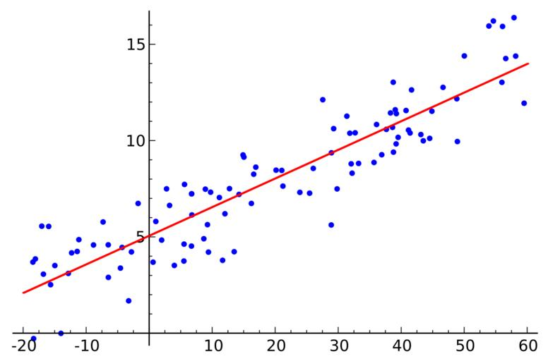
There are two variables in this diagram - X and Y.

A linear equation is created and fit on the dataset. This equation will predict variable Y given variable X.

Variable Y is called the dependent variable, and X is the independent variable.

The dependent variable is predicted by the independent variable.

For example: Tom wants to predict house prices given their area. In this case, the house price is the dependent variable, and the area is the independent variable.

Simple vs Multiple Linear Regression

A simple linear regression model only involves one dependent variable and one independent variable.

Example: Predicting house price based on its area.

In a multiple linear regression model, there are more than one independent variables.

Example: Predicting house price based on its area, number of bedrooms, floors, etc.

Linear Function

Take a look at the above diagram again.

The equation of this line is y = mx + c. This is called a linear function.

Here, y is the dependent variable, x is the independent variable, m is the slope of the line, and c is the y intercept.

If you plug in any value of x into this equation, you can come up with the output prediction y.

How is this line fit onto the data?

The linear function is also called the line of best fit.

We want a line that fits all the data points as well as possible so that we can come up with accurate predictions.

The most common method of fitting this line onto data is called the least-squares method.

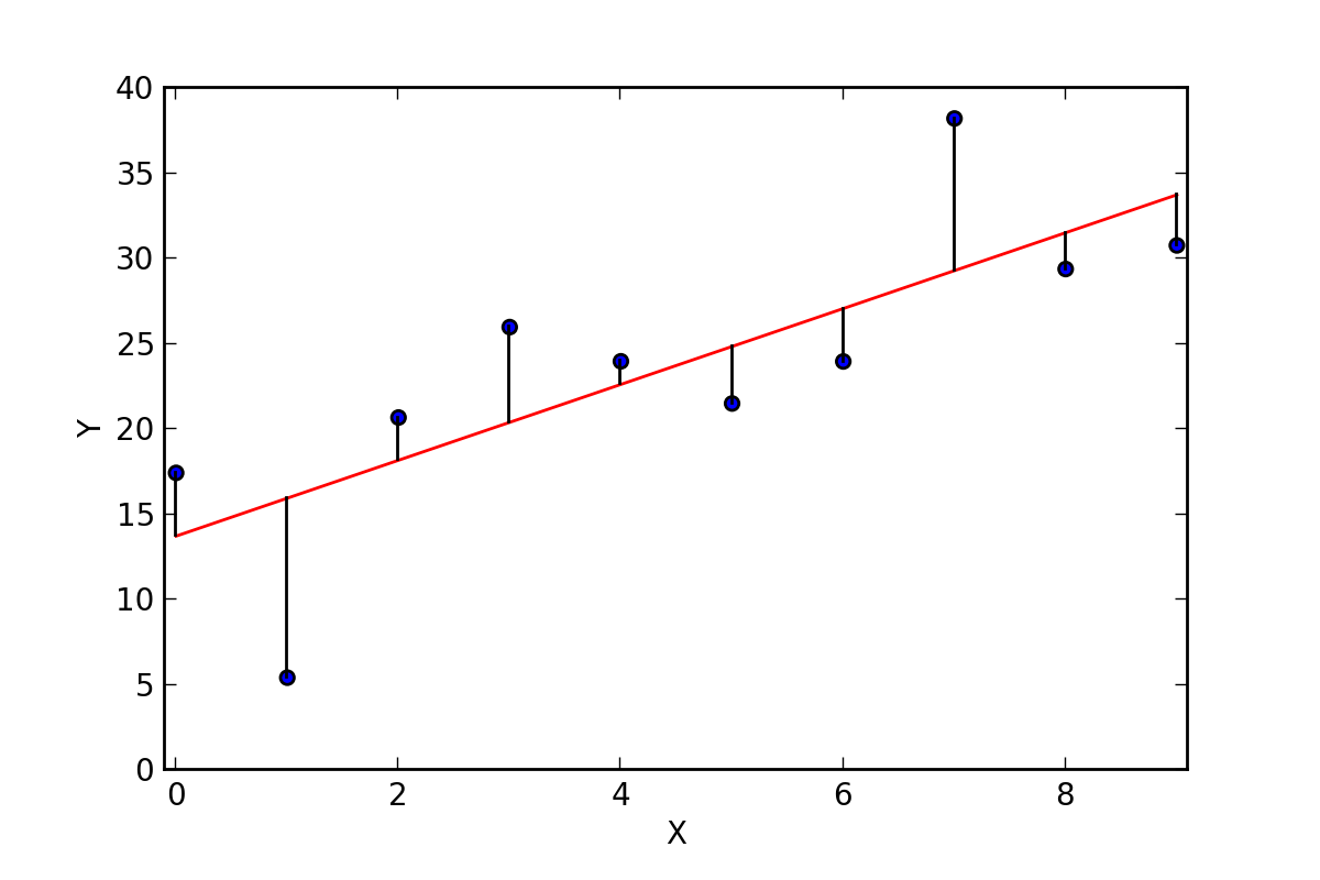
Take a look at the image above.

The least-squares method will fit the red line onto the data such that the sum of squared error between the predictions and true values are minimized.

For example, take the first data point in the diagram. Its true y value is 17, and the predicted value on the line is around 14.

For the second data point, the true y value is around 5, and the predicted value is around 16.

The difference of all these values will be obtained, and that is the error. Then, we square these errors and take its sum, which looks like this:

(17-14)² + (5-16)² + (21-17)² + ...

The result that we get should be as small as possible, as we want to minimize these residuals as much as we can.

If you've built a linear regression model using computer packages in the past, the linear function is inbuilt into these programs. All you have to do is run a few lines of code, and the program will calculate the best fit line for you. This will be demonstrated with code snippets in this tutorial.

When to use linear regression?

Only use linear regression when there is a linear relationship between your dependent and independent variable.

To identify whether the variables X and Y have a linear relationship, first create a scatterplot to visualize the data.

Scenario 1

Taking a look at the picture above, we can see that there is a linear relationship between these two variables. We can make highly accurate predictions of Y given values of X.

Scenario 2

In this diagram, however, we can see that there is no linear relationship between these two variables. In this case, a linear regression model will probably not perform too well.

Later in this tutorial, Python codes to create a scatterplot will be provided.

Another useful measure to see if variables have a strong linear relationship is correlation.

If variables are highly correlated, then the independent variable is useful in predicting the dependent variable.

Correlation

Correlation quantifies the strength of the relationship between variables X and Y.

If two variables X and Y have high correlation, it means that the relationship between these variables are stronger.

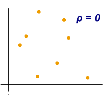
The correlation coefficient ranges from -1 to 1. A value of 0 indicates that X and Y have no correlation at all, and there is no linear relationship.

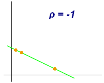
A value of -1 indicates that there is a perfect negative linear relationship between X and Y.

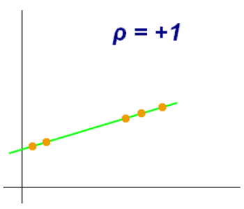
A value of +1 indicates that there is a perfect positive linear relationship between X and Y.

This means that the closer the correlation coefficient is to zero, the weaker the relationship between variables.

The closer the correlation coefficient is to +1 or -1, the stronger the relationship between the variables.

Example:

a) The correlation coefficient between X and Y in this diagram is zero. There is no linear relationship here.

b) The correlation coefficient between X and Y in this case is +1. There is a perfect positive linear relationship between the variables.

c) The correlation coefficient between X and Y in this case is -1. There is a perfect negative linear relationship between the variables.

R-Squared

The square of the correlation coefficient is the R-squared value.

This value tells us how much of the variance in Y (the dependent variable) can be explained by the variance in X (the independent variable).

For example, if the correlation coefficient between X and Y is 0.8, then the R-squared value is 80%. This means that 80% of the variation in Y can be explained by the variation in X.

The R-squared value can be defined by the following formula:

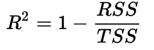
Here, RSS is the sum of square of residuals, and TSS is the total sum of squares.

RSS is the same as SSE, or sum or squared error that we computed earlier.

It is defined as the sum ofsquares of predicted values minus their true value.

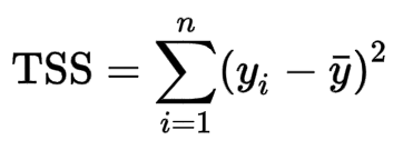
TSS, or the total sum of squares is defined as the sum of squares of true values minus their mean.

In other words, we find the true Y values of all the data points, and then subtract with the average of all these Y values.

The equation to find the total sum of squares looks like this:

If you want to find out how good the independent variable is at explaining the variance of the dependent variables, then all you need to do is compute the R-squared value.

This value can be computed with just one line of code using R/Python packages, so you won't have to do any of this manual calculation by hand.

Linear Regression in Python

Now, we will build a linear regression model in Python. You can use this tutorial as starter code for future regression problems.

We will be doing an example to get acquainted with all the concepts you have learnt so far in this tutorial.

Here is a link to the dataset we will be using. Make sure to download the dataset before starting the tutorial.

Pre-requisites

The following Python libraries will be used in this tutorial - Pandas, Numpy and Scikit-Learn.

Make sure to have these installed before you start to code along.

Step 1: Imports

First, lets import all the necessary libraries:

import pandas as pd
import numpy as np
from sklearn.linear_model import LinearRegression
from sklearn.model_selection import train_test_split
from sklearn.metrics import mean_squared_error
import math

Step 2: Read the data

Now, read the .csv file into a dataframe with Pandas:

import pandas as pd
df = pd.read_csv('winequality-red.csv',sep=';')

Step 3: Examining the data

Lets first check the head of the dataframe. We want to get an understanding of all the different variables present.

df.head()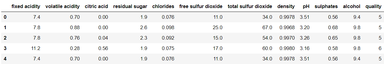

Observe that there are 12 variables in the dataframe.

Independent variables: fixed acidity, volatile acidity, citric acid, residual sugar, chlorides, free sulfur dioxide, total sulfur dioxide, density, pH, sulphates, alcohol.

Dependent variable: quality

All other variables in the dataset will be used to predict wine quality.

Step 4: Feature Selection

Sometimes, not all features in the dataset are useful in explaining the dependent variable.

Feature selection is the most important step towards building any machine learning model, since a model is only as good as the features used to create it.

In this case, we will do feature selection with a concept we learnt about earlier - correlation.

We will take a look at the correlation between every independent variable and wine quality.

Then, we can choose to keep variables that have high correlation with wine quality, and drop the rest.

This is a simple feature selection technique, but is very helpful in eliminating features that aren't useful in explaining the target variable. Reducing the feature space also helps to save time and cost, especially when dealing with large datasets.

Finding the correlation between all independent variables and wine quality:

correlations = df.corr()['quality'].drop('quality')
print(correlations)

You should see the following output:

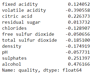
From here, we can see that alcohol has the highest correlation with the target variable.

Remember that correlation values can range from -1 to +1, where -1 indicates perfect negative correlation and +1 indicates perfect positive correlation. This is called Pearson's correlation coefficient.

Now, lets write some code removes variables with weak correlations.

For this model, I will define weak correlation as follows:

Variables that have a correlation coefficient ranging from 0 to 0.10 (weak positive correlation)
Variables that have a correlation coefficient ranging from -0.10 to 0 (weak negative correlation)

list1 = []
for i in range(len(correlations)):
    if((correlations[i]>=0) & (correlations[i]<=0.10)):
        list1.append(i)
    elif((correlations[i]<=0) & (correlations[i]>=-0.10)):
        list1.append(i)
        
print(list1)

The codes above should render the following list as output: [3, 5, 8].

This means that variables 3, 5 and 8 (residual sugar, free sulfur dioxide, pH) have low correlations with the output, and aren't very useful towards predicting wine quality.

We need to drop these variables before building the model.

Step 5: Model Building

First, lets split the data into train and test datasets. Remember, we need to drop the variables with low correlation first:

X = df.drop(['quality','residual sugar','free sulfur dioxide','pH'],axis=1)
y = df['quality']
X_train, X_test, y_train, y_test = train_test_split(X, y, test_size=0.33, random_state=42)

Now, lets instantiate a linear regression model and fit it onto the training set:

lm = LinearRegression()
lm.fit(X_train, y_train)

Then, we can make predictions on the test set with this data:

preds = lm.predict(X_test)

Step 6: Evaluation

Now, we can evaluate the performance of the model we just built.

There are many different metrics we can use to do this, some of which we learnt in previous sections (such as R-squared and SSE).

Here, we will look at a metric called the Root Mean Squared Error (RMSE).

The Root Mean Squared Error looks at the squared difference between the true and predicted value. Then, it takes the average difference across the entire dataset and squares it.

The formula for calculating the Root Mean Squared Error is as follows:

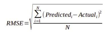
Now, lets write some code to calculate the RMSE of our model:

mse = mean_squared_error(y_test, preds)
print(math.sqrt(mse))

You should get a RMSE value of around 0.65.

Additional Resources

There is a lot more to linear regression than what was explained in this article. If you are interested in learning more about regression techniques, I suggest the following learning resources: