RFM Analysis with Python

RFM modelling is a marketing analysis technique used to evaluate a customer's value. The RFM model is based on three factors:

• Recency: How recently a customer has made a purchase
• Frequency: How often a customer makes a purchase
• Monetary Value: How much money a customer spends on purchases

An RFM model comes up with numeric values for the three measures above. These values help companies better understand customer potential.

For example

If a customer made a purchase daily from Starbucks in the past year and hasn't bought anything in the last month, they could be moving to a competitor brand. They might have made a switch to The Coffee Bean and Tea Leaf now due to better deals or convenience.

Starbucks can then target these customers and come up with a marketing strategy to win them back.

In this article, I will show you how to build an RFM model with Python. We will use a dataset that contains over 4000 unique customer IDs, and will assign RFM values to each of these customers.

Download the dataset from Kaggle to get started. Make sure you have a Python IDE installed on your device, along with the Pandas library.

Step 1

Read the downloaded dataset with the following lines of code:

import pandas as pd

df2 = pd.read_csv('data.csv',encoding='unicode_escape')

Now, let's look at the head of the data frame:

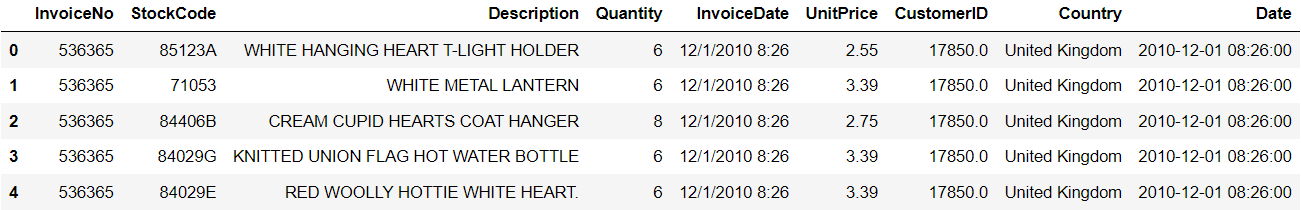
df.head()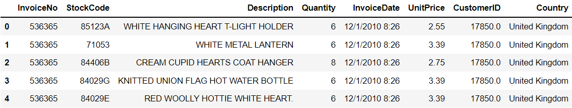

For this analysis, we will only be using four columns: Quantity, InvoiceDate, UnitPrice, CustomerID.

Step 2

Let's start by calculating the value of M - monetary value. This is the simplest value to calculate. All we need to do is calculate the total amount spent by each customer.

To do this, we need to use the columns UnitPrice and Quantity. We will multiply these values first, to get the total amount spent by each customer for each transaction.

Here's the code to do this:

df['Total'] = df['Quantity']*df['UnitPrice']

Great!

Let's check the head of the data frame now:

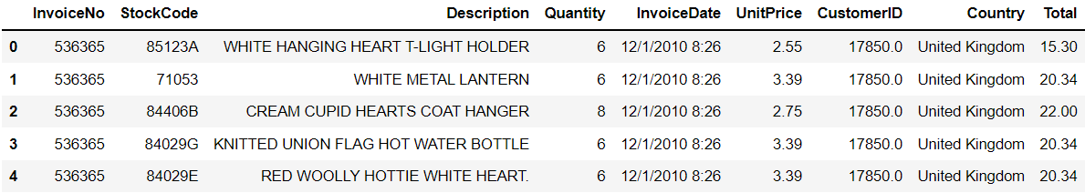
We can see a new column with the total amount spent for each transaction.

Now, we need to find the total amount spent by the same customer throughout the entire dataset. We can do this with the following lines of code:

m = df.groupby('CustomerID')['Total'].sum()
m = pd.DataFrame(m).reset_index()

Looking at the head of our new data frame, we can see this:

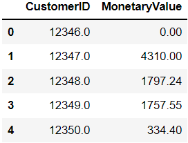
Great! We have now successfully calculated the monetary value of each customer in the data frame.

Step 3

Now, let's calculate the frequency. We want to find the number of times each customer has made a purchase.

Let's take a look at the data frame again to see how we can do this:

To find the number of times each customer was seen making a purchase, we need to use the columns CustomerID and InvoiceDate.

We need to calculate the number of unique dates each customer was seen making a purchase.

To do this, run the following lines of code:

freq = df.groupby('CustomerID')['InvoiceDate'].count()
f = pd.DataFrame(freq).reset_index()

Taking a look at the head of the data frame, you should see this:

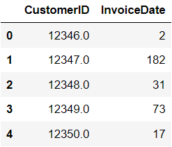
Great! We have successfully come up with a quantitative measure of frequency for each customer in the data frame.

Step 4

Finally, we can calculate the recency of each customer in the data frame.

To calculate recency, we need to find the last time the person was seen making a purchase. Was it a year ago? Months ago? Or a few days back?

To find this value, we need to use the CustomerID and InvoiceDate column. We first need to find the latest date each customer was seen making a purchase. Then, we need to assign some quantitative value to this date.

For example, if customer A was seen making a purchase two months ago and customer B was seen making a purchase two years ago, we need to assign a higher recency value to customer A.

To do this, we first need to convert the InvoiceDate column to a datetime object. Run the following lines of code:

df['Date']= pd.to_datetime(df['InvoiceDate'])

Let's take a look at the head of the data frame again:

Notice that we now have a new 'Date' column.

Now, need to find the most recent date each customer was seen making a purchase.

To do this, we need to assign a rank to all the dates for each CustomerID. The most recent date will be ranked as 1, second most recent date as 2, and so on.

Run the following lines of code:

df['rank'] = df.sort_values(['CustomerID','Date']).groupby(['CustomerID'])['Date'].rank(method='min').astype(int)

Taking a look at the head of the data frame, we can see this:

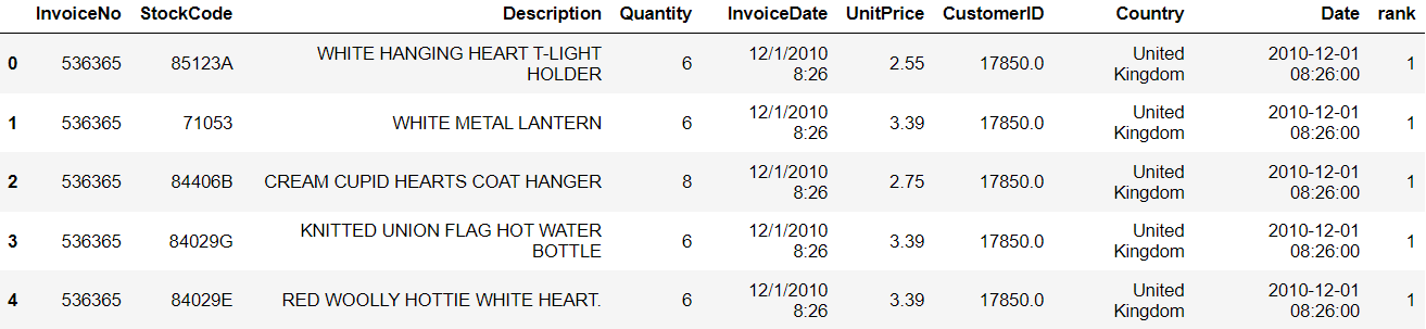
Now we have different ranks based on the time the customer was seen making a purchase. The most recent purchase has a rank of 1.

Let's now filter the data frame and get rid of all the other purchases. We only need to keep the most recent ones:

recent = df[df['rank']==1]

Perfect!

Now all we need to do is come up with a quantitative recency value. This means that a person seen one day ago will be given a higher recency value as compared to someone seen one week ago.

To do this, let's just calculate the difference between every date in the data frame and the earliest date. This way, more recent dates will have a higher value.

Run the following lines of code:

recent['recency'] = recent['Date'] - pd.to_datetime('2010-12-01 08:26:00')

Now, let's take a look at the head of the data frame:

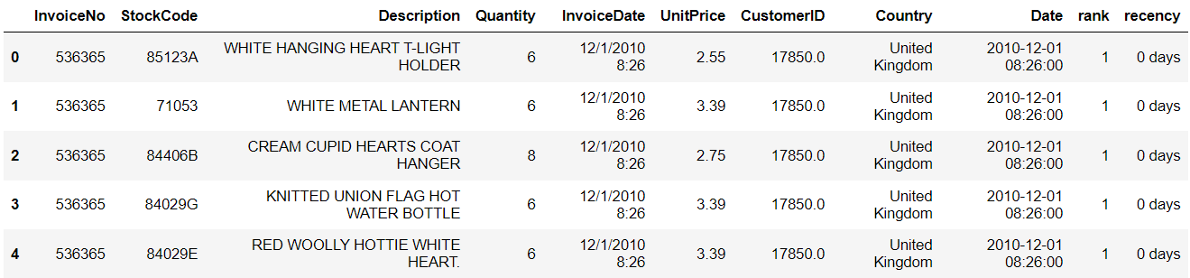
Notice that we have a new column labelled 'recency,' and the number of days from the oldest date in the dataset has been calculated. A value of 0 days indicates lowest recency.

We can now convert the recency values into numeric. To do this, run the following lines of code:

def recency(recency):
    res = str(recency).split(' ')[0]
    return(int(res))
    
recent['recency'] = recent['recency'].apply(recency)

Finally, notice that the data frame above has many duplicate values for each CustomerID. This is because the breakdown is by product, and the same customers purchased multiple products at the same time.

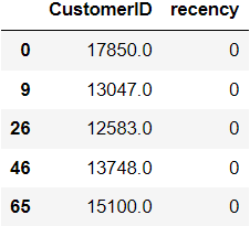
Let's select only the CustomerID and recency columns and remove duplicates:

recent = recent[['CustomerID','recency']]
recent = recent.drop_duplicates()

Taking a look at the head of the data frame, you should see this:

Step 5

We're now done calculating RFM values. We have the results stored in separate data frames, so let's merge them together:

finaldf = f.merge(m,on='CustomerID').merge(recent,on='CustomerID')

Let's now take a look at the head of the final data frame:

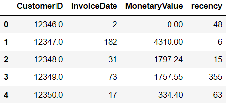
That's it!

We have successfully managed to append RFM values to each customer ID in the dataset.

We can come up with customer insights based on these calculations, or build some sort of clustering model to group similar customers together.

If you managed to run the codes above successfully, then try going a step further and normalize these values. RFM values are usually presented on a scale of 1-5, so you can create bins for each of these values and group them together.

Thanks for reading, I hope you enjoyed this tutorial.